Taufactor Overview

TauFactor is an open-source, GPU accelerated microstructural analysis tool for extracting metrics from voxel based data, including volume fractions, interfacial areas and effective transport properties.

Tortuosity solvers

The tortuosity factor \(\tau\) is a morphological parameter that defines the reduction in transport arising from constrictions and tortuos pathways.

The main output of the solve function is a scalar tortuosity \(\tau\) or the spatially resolved \(\tau(x)\). In the following example, s.tau is the classical tortuosity factor \(\tau_\text{c}\), a measure of the reduction in diffusive transport caused by convolution in the geometry of the material. s.D_eff is the effective diffusivity resulting from the tortuous nature of the material. The relationship between these values is given by:

\(D_{eff}=D\frac{\epsilon}{\tau_\text{c}}\)

For more see Cooper et al.

import taufactor as tau
import tifffile

# Load segmented image, in this case with
# labels {"pore":0, "NMC":85, "CBD":170}
img = tifffile.imread('electrode.tiff')
s = tau.Solver(img==0)
tau_x = s.solve()

print(f"tau = {s.tau[0]:.4f}, D_eff = {s.D_eff[0]:.4f}*D_0")

converged to: [2.0776296] after: 700 iterations in: 10.9197s (0.0156 s/iter)
GPU-RAM currently 339.74 MB (max allocated 540.80 MB; 547.36 MB reserved)
tau = 2.0776, D_eff = 0.2166*D_0

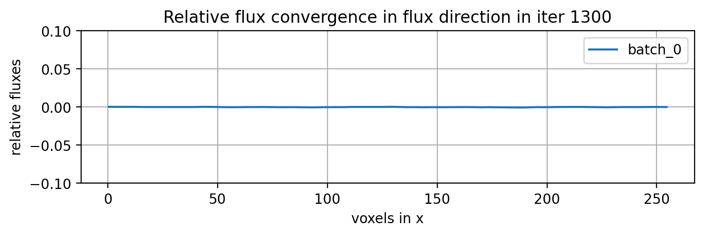
The iteration limit, convergence criteria and verbosity of the solver can be adjusted. Setting verbose='per_iter' logs the output of the solver every 100 steps whilst solving. The option verbose='plot' plots the relative flux convergence every 100*plot_interval steps. verbose='None disables all written output. The conv_crit controls the value at which convergence is met.

s = tau.Solver(img==0)
tau_x = s.solve(verbose='plot', plot_interval=1, conv_crit=1e-3)

Iter: 1300, conv error: 9.581E-04, tau: 2.07716 (batch element 0)

converged to: [2.0771587] after: 1300 iterations in: 21.3182s (0.0164 s/iter)
GPU-RAM currently 339.74 MB (max allocated 540.80 MB; 685.77 MB reserved)

By default, the direction of transport is the first index of the loaded image. If a different direction is required, the image must be permuted before solving. To visualise this and give guidance, the utility function flux_direction can be used.

from taufactor.utils import flux_direction
figure = flux_direction(img)

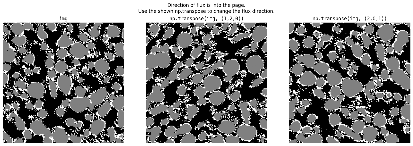
Therefore, to solve the simulation in the y direction we can run

import numpy as np

s = tau.Solver(np.transpose(img, (1,2,0))==0)
tau_y = s.solve(verbose=None)

print(f"Tau in y-direction is {s.tau[0]:.4f}")

Tau in y-direction is 2.0766

Other Solvers

Periodic solver

The periodic solver applies periodic boundary conditions instead of mirror boundaries.

s = tau.PeriodicSolver(img==0)
s.solve()

Anisotropic solver

The anisotropic solver accounts for non-cubic voxels such as commonly encountered in FIB-SEM stacks (different spacing dz in cutting direction). If dz is twice as large as the pixel resolution dx=dy, set the spacing=(1,1,2).

s = tau.AnisotropicSolver(img==0, spacing=(1,1,2))
s.solve()

Multi-phase solver

The multi-phase solver allows for more than 2 conductive phases per image. The conductivity of each phase is given as an input to the solver along with the phase label

# assign conductivity values, where key is segmented label in 'img'
# and value is conductivity
cond = {1:0.32, 2:0.44}

# create a multiphase solver object and set an iteration limit
s = tau.MultiPhaseSolver(img, cond=cond, iter_limit=1000)
# call solve function
s.solve()

Metrics

Metrics can be calculated using the metrics module

from taufactor.metrics import *

Volume fraction

Volume fraction is calculated for each phase in a segmented image:

from taufactor.metrics import volume_fraction

# calculate the volume fraction
vf = volume_fraction(img)

# consider a three phase image with pore, particle and binder
# where 0, 1, 2 correspond to pore, particle and binder respectively
# calculate the volume fraction
vf = volume_fraction(img, phases={'pore':0, 'particle':1, 'binder':2})

Specific surface area

Per default, the specific surface area is calculated for each phase in a segmented image. Alternatively, the phases can be specified as phases={‘phase1’: 0, …}. The method to compute surface area can be chosen as ‘face_counting’, ‘marching_cubes’ or ‘gradient’. A detailed comparison of these methods can be found in Daubner et al.. While face_counting is the fastest, the gradient method yields more accurate results for curved geometries.

from taufactor.metrics import specific_surface_area
# calculate the surface area of all phases in an image
sa = specific_surface_area(img)

# Surface area of a particular phase on anisotropic voxel grid (e.g. FIB-SEM data)
sa = specific_surface_area(img, spacing=(1,1,3), phases={'pore': 0})

# consider a three phase image with pore, particle and binder
# where 0, 1, 2 correspond to pore, particle and binder respectively
# Use voxel face counting for fastest computation
labels={'pore':0, 'particle':1, 'binder':2}
sa = surface_area(img, phases=labels, method='face_counting')

Triple phase boundary

Triple phase boundary is calculated on a segmented image with exactky three phases. The value returned is the fraction of triple phase edges with respect to the total number of edges

from taufactor.metrics import triple_phase_boundary
# calculate the triple phase boundareies
tpb = triple_phase_boundary(img)