Appendix: Benchmarking Solvers

Benchmarks on simple test structures can be used for

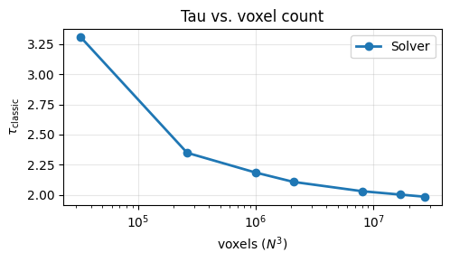
1. Investigation of convergence of the classical tortuosity factor with increasing voxel count. This addresses pixelation artifacts.

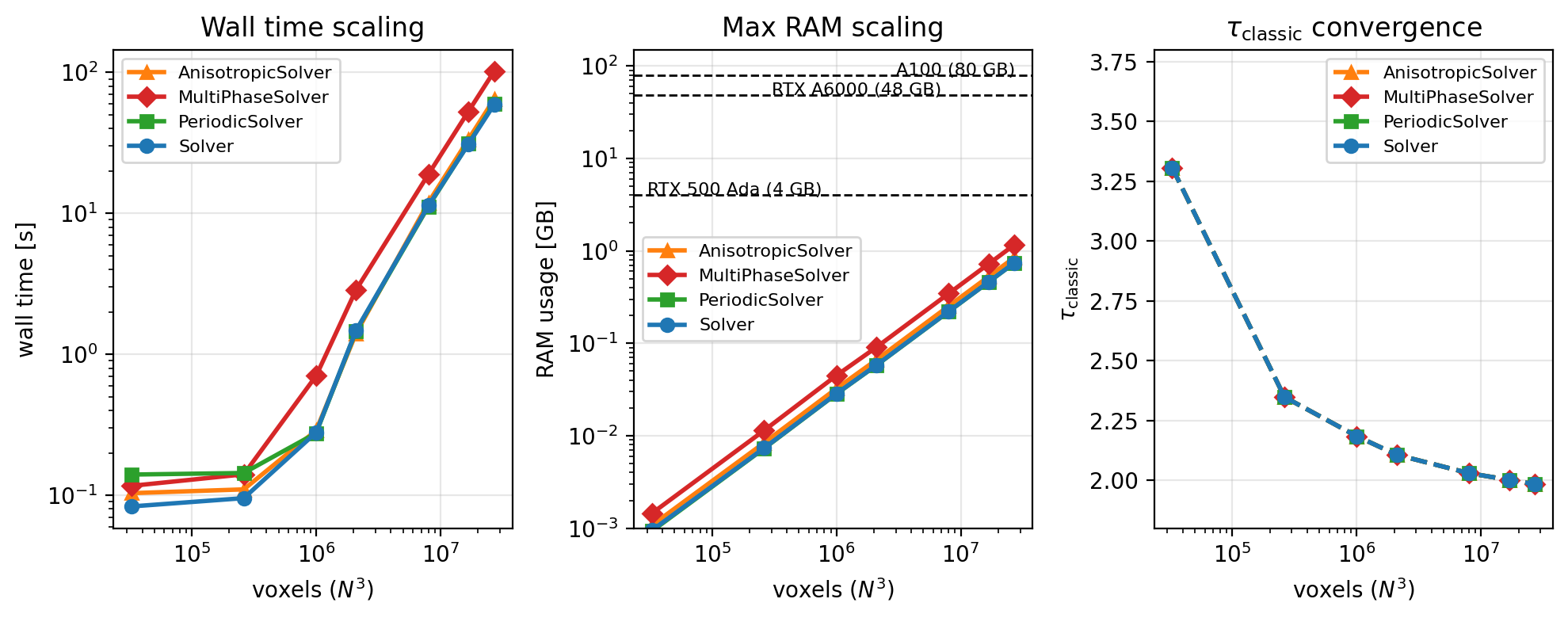
2. Cross-validation between various solvers to check consistency and different wall-time and RAM scaling (Solver, PeriodicSolver, AnisotropicSolver, MultiPhaseSolver).

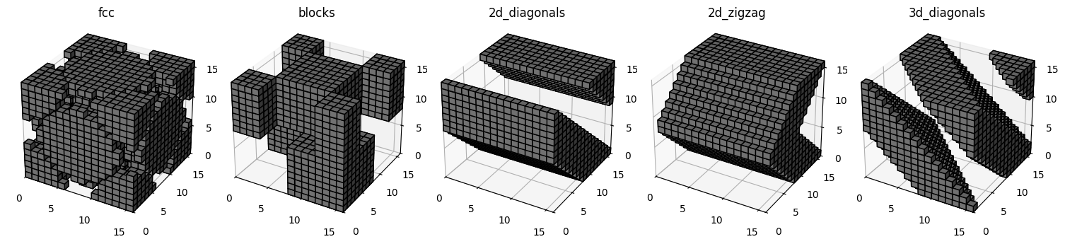
In utils.py, various test structures are predefined which can directly be called by the run_benchmark_study function in benchmark.py. We first visualise the various test structures…

from taufactor.utils import create_fcc_cube, \
    create_stacked_blocks, create_2d_diagonals, \
    create_3d_diagonals, create_2d_zigzag
import matplotlib.pyplot as plt
import numpy as np

Nx = 16
fields = {}

fields["fcc"] = create_fcc_cube(Nx)
fields["blocks"] = create_stacked_blocks(Nx, features=1)
fields["2d_diagonals"] = create_2d_diagonals(Nx, features=1)
fields["2d_zigzag"] = create_2d_zigzag(Nx, features=1)
fields["3d_diagonals"] = create_3d_diagonals(Nx, features=1)

fig, axes = plt.subplots(nrows=1, ncols=5, figsize=(15, 4), dpi=100)
for i, structure in enumerate(fields.keys()):
    axes[i].remove()
    axes[i] = fig.add_subplot(1, 5, i + 1, projection='3d')
    axes[i].voxels(np.transpose(fields[structure], (2,1,0))==1, facecolors='gray', edgecolor='black', alpha=1.0)
    axes[i].set_zlim(0, Nx)
    axes[i].set_aspect('equal')
    axes[i].set_title(structure)
    axes[i].set_xlim(0, Nx)
    axes[i].set_ylim(0, Nx)
plt.tight_layout()
plt.show()

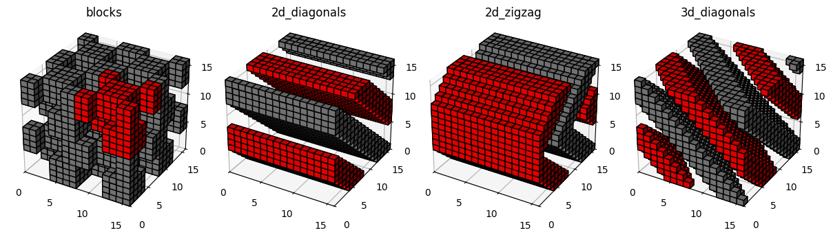
It is also possible to create the blocks, 2d_diagonals, 2d_zigzag and 3d_diagonals with multiple features in a repeating pattern e.g.

from taufactor.metrics import label_periodic
from scipy.ndimage import generate_binary_structure

fields = {}
features = 2
fields["blocks"] = create_stacked_blocks(Nx, features=features)
fields["2d_diagonals"] = create_2d_diagonals(Nx, features=features)
fields["2d_zigzag"] = create_2d_zigzag(Nx, features=features)
fields["3d_diagonals"] = create_3d_diagonals(Nx, features=features)

fields["blocks"][Nx//2:,:Nx//2,Nx//2:] *= 2
connectivity = generate_binary_structure(3, 1)
fields["2d_diagonals"] = label_periodic(fields["2d_diagonals"], 1, connectivity, periodic=(False, True, True))[0]
fields["2d_zigzag"] = label_periodic(fields["2d_zigzag"], 1, connectivity, periodic=(False, True, True))[0]
fields["3d_diagonals"] = label_periodic(fields["3d_diagonals"], 1, connectivity, periodic=(False, True, True))[0]

colors = ['white', 'gray', 'red', 'blue', 'green']
fig, axes = plt.subplots(nrows=1, ncols=4, figsize=(15, 4), dpi=100)
for i, structure in enumerate(fields.keys()):
    axes[i].remove()
    axes[i] = fig.add_subplot(1, 5, i + 1, projection='3d')
    for j in np.unique(fields[structure]):
        if j>0:
            axes[i].voxels(np.transpose(fields[structure], (2,1,0))==j, facecolors=colors[j], edgecolor='black', alpha=1.0)
    axes[i].set_zlim(0, Nx)
    axes[i].set_aspect('equal')
    axes[i].set_title(structure)
    axes[i].set_xlim(0, Nx)
    axes[i].set_ylim(0, Nx)
plt.tight_layout()
plt.show()

Tau Convergence vs. Voxel Count on FCC cube

from taufactor.benchmark import run_benchmark_study
import pandas as pd

Ns = [32, 64, 100, 128, 200, 256, 300]
res = run_benchmark_study(
    Ns=Ns,
    devices=['cuda'],
    conv_crit_values=[1e-3],
    structure='fcc',
    solver='Solver',
    write_file=False,
)

df_solver = pd.DataFrame(res).sort_values('N').reset_index(drop=True)
df_solver

	N	structure	solver	device	conv_crit	total_time	solve_time	iterations	taufactor	torch_cur	torch_max	torch_res
0	32	fcc	Solver	cuda	0.001	0.232843	0.104405	400	3.307094	0.71	0.97	2.10
1	64	fcc	Solver	cuda	0.001	0.102649	0.082804	500	2.348118	5.45	7.54	27.26
2	100	fcc	Solver	cuda	0.001	0.359405	0.308809	800	2.184316	21.22	29.22	44.04
3	128	fcc	Solver	cuda	0.001	1.537179	1.453016	1000	2.106697	42.74	59.52	85.98
4	200	fcc	Solver	cuda	0.001	11.482289	11.105710	1500	2.029747	163.11	227.11	236.98
5	256	fcc	Solver	cuda	0.001	31.583841	30.962704	2000	2.001894	339.74	473.96	480.25
6	300	fcc	Solver	cuda	0.001	60.363106	59.183771	2400	1.984324	546.30	762.30	773.85

fig, ax = plt.subplots(figsize=(5, 3), dpi=100)
x_voxels = df_solver['N'] ** 3
ax.plot(x_voxels, df_solver['taufactor'], marker='o', linewidth=2, color='#1f77b4', label='Solver')
ax.set_xscale('log')
ax.set_xlabel('voxels ($N^3$)')
ax.set_ylabel('$\\tau_\\text{classic}$')
ax.set_title('Tau vs. voxel count')
ax.grid(True, alpha=0.3)
ax.legend(loc='best')
plt.tight_layout()
plt.show()

Solver Cross-Comparison (Wall Time and RAM)

solver_specs = [
    {'solver': 'Solver', 'label': 'Solver', 'solver_kwargs': {}},
    {'solver': 'PeriodicSolver', 'label': 'PeriodicSolver', 'solver_kwargs': {}},
    {'solver': 'AnisotropicSolver', 'label': 'AnisotropicSolver', 'solver_kwargs': {'spacing': (1.0, 1.0, 1.0)}},
    {'solver': 'MultiPhaseSolver', 'label': 'MultiPhaseSolver', 'solver_kwargs': {}},
]

all_rows = []
for spec in solver_specs:
    print(f"Running {spec['label']}...")
    rows = run_benchmark_study(
        Ns=Ns,
        devices=['cuda'],
        conv_crit_values=[1e-3],
        structure='fcc',
        solver=spec['solver'],
        solver_kwargs=spec['solver_kwargs'],
        outfile='fcc_benchmark_results.txt',
        write_file=True,
    )
    for r in rows:
        r['solver_label'] = spec['label']
    all_rows.extend(rows)

df_compare = pd.DataFrame(all_rows)
# df_compare

Running Solver...
Running PeriodicSolver...
Running AnisotropicSolver...
Running MultiPhaseSolver...

colors = {
    'Solver': '#1f77b4',
    'PeriodicSolver': '#2ca02c',
    'AnisotropicSolver': '#ff7f0e',
    'MultiPhaseSolver': '#d62728',
}
markers = {
    'Solver': 'o',
    'PeriodicSolver': 's',
    'AnisotropicSolver': '^',
    'MultiPhaseSolver': 'D',
}

fig, (ax1, ax2, ax3) = plt.subplots(1, 3, figsize=(10, 4), dpi=200)
for label, g in df_compare.groupby('solver_label'):
    g = g.sort_values('N')
    x = g['N'] ** 3
    ax1.loglog(
        x, g['solve_time'], marker=markers.get(label, 'o'), linewidth=2,
        color=colors.get(label), label=label
    )
    ax2.loglog(
        x, g['torch_max']/1024, marker=markers.get(label, 'o'), linewidth=2,
        color=colors.get(label), label=label
    )
    ax3.semilogx(
        x, g['taufactor'], marker=markers.get(label, 'o'), linewidth=2,
        color=colors.get(label), label=label, linestyle='--'
    )

# Hardware reference lines when using CUDA
for x, y, txt in [(3e4, 4, 'RTX 500 Ada (4 GB)'), (3e5, 48, 'RTX A6000 (48 GB)'), (3e6, 80, 'A100 (80 GB)')]:
    ax2.axhline(y, color='black', linestyle='--', linewidth=1)
    ax2.text(x, y, txt, fontsize=8, color='black')

ax1.set_xlabel('voxels ($N^3$)')
ax1.set_ylabel('wall time [s]')
ax1.set_title('Wall time scaling')
ax1.legend(loc='best', fontsize=8)
ax1.grid(True, alpha=0.3)

ax2.set_xlabel('voxels ($N^3$)')
ax2.set_ylabel('RAM usage [GB]')
ax2.set_title('Max RAM scaling')
ax2.legend(loc='best', fontsize=8)
ax2.set_ylim(0.001, 150)
ax2.grid(True, alpha=0.3)

ax3.set_xlabel('voxels ($N^3$)')
ax3.set_ylabel('$\\tau_\\text{classic}$')
ax3.set_title('$\\tau_\\text{classic}$ convergence')
ax3.legend(loc='best', fontsize=8)
ax3.set_ylim(1.8, 3.8)
ax3.grid(True, alpha=0.3)

plt.tight_layout()
plt.show()

summary = (
    df_compare.groupby('solver_label', as_index=False)
    .agg(
        wall_time_mean_s=('solve_time', 'mean'),
        wall_time_max_s=('solve_time', 'max'),
        ram_peak_MB=('torch_max', 'max'),
        max_iterations=('iterations', 'max'),
    )
    .sort_values('wall_time_mean_s')
)
summary

	solver_label	wall_time_mean_s	wall_time_max_s	ram_peak_MB	max_iterations
3	Solver	14.767117	59.091109	762.30	2400
2	PeriodicSolver	14.917869	59.956331	760.20	2400
0	AnisotropicSolver	16.008609	64.687983	870.30	2400
1	MultiPhaseSolver	25.325081	101.644147	1192.92	2400

Multiphase Diffusivity Study

It is furthermore possible to create your own test geometries and run a benchmark study with them. To do so, you need to write a function and pass it to the benchmark study call. We combine this here with testing specifics of the multi-phase solver.

from taufactor.utils import create_2d_zigzag

def multi_zigzag(Nx):
    geom = create_2d_zigzag(Nx, features=1)
    N2 = Nx // 2
    geom[:N2, :, :][geom[:N2, :, :] == 1] = 2
    return geom

all_rows = []
diffusivities = [0.1, 0.5, 1.0, 2.0, 10.0]

for c in diffusivities:
    rows = run_benchmark_study(
        Ns=[64],
        solver='MultiPhaseSolver',
        solver_kwargs={'diffusivities': {0:0, 1: 1.0, 2: c}},
        structure=multi_zigzag,
        write_file=False,
    )
    for r in rows:
        r['diffusivity'] = c
    all_rows.extend(rows)

df_ratio = pd.DataFrame(all_rows).sort_values('diffusivity').reset_index(drop=True)
df_ratio

	N	structure	solver	device	conv_crit	total_time	solve_time	iterations	taufactor	torch_cur	torch_max	torch_res	diffusivity
0	64	multi_zigzag	MultiPhaseSolver	cuda	0.001	0.361350	0.309471	600	4.863471	8.54	11.69	29.36	0.1
1	64	multi_zigzag	MultiPhaseSolver	cuda	0.001	0.226141	0.173996	500	1.808737	8.54	11.69	29.36	0.5
2	64	multi_zigzag	MultiPhaseSolver	cuda	0.001	0.149334	0.128130	400	1.607159	8.54	11.69	29.36	1.0
3	64	multi_zigzag	MultiPhaseSolver	cuda	0.001	0.181795	0.151589	500	1.808737	8.54	11.69	29.36	2.0
4	64	multi_zigzag	MultiPhaseSolver	cuda	0.001	0.171382	0.153869	600	4.863406	8.54	11.69	29.36	10.0

The results of this first study show that the tortuosity factor of multiphase simulations depends on the ratio of diffusivities/conductivities. When \(D_a\) is kept at \(1\) and \(D_b\in[0.1, 0.5, 1.0, 2.0, 10.0]\), we observe a symmetry in \(\tau_\text{c}\) values.

In the next study, we create multiple diagonals, which are labelled as \(1\) and \(2\) (see the Figure above with grey and red features). Even though the effective diffusivity depends on the actual value of \(D_b\), the tortuosity factor does not and is, in this case of parallel conducting channels, a purely geometric quantity.

from taufactor.utils import create_2d_diagonals

def multi_diagonal(Nx):
    geom = create_2d_diagonals(Nx, features=2)
    geom = label_periodic(geom, 1, connectivity, periodic=(False, True, True))[0]
    return geom

all_rows = []
diffusivities = [0.1, 0.5, 1.0, 2.0, 10.0]

for c in diffusivities:
    rows = run_benchmark_study(
        Ns=[64],
        solver='PeriodicMultiPhaseSolver',
        solver_kwargs={'diffusivities': {0:0, 1:1, 2:c, 3:1, 4:c}},
        structure=multi_diagonal,
        write_file=False,
    )
    for r in rows:
        r['diffusivity'] = c
    all_rows.extend(rows)

df_ratio = pd.DataFrame(all_rows).sort_values('diffusivity').reset_index(drop=True)
df_ratio

	N	structure	solver	device	conv_crit	total_time	solve_time	iterations	taufactor	torch_cur	torch_max	torch_res	diffusivity
0	64	multi_diagonal	PeriodicMultiPhaseSolver	cuda	0.001	0.239640	0.220841	500	2.010120	8.54	11.69	29.36	0.1
1	64	multi_diagonal	PeriodicMultiPhaseSolver	cuda	0.001	0.260428	0.235632	500	2.010121	8.54	11.69	29.36	0.5
2	64	multi_diagonal	PeriodicMultiPhaseSolver	cuda	0.001	0.241486	0.218591	500	2.010121	8.54	11.69	29.36	1.0
3	64	multi_diagonal	PeriodicMultiPhaseSolver	cuda	0.001	0.209310	0.188352	500	2.010121	8.54	11.69	29.36	2.0
4	64	multi_diagonal	PeriodicMultiPhaseSolver	cuda	0.001	0.208770	0.188987	500	2.010121	8.54	11.69	29.36	10.0

This multi-phase \(\tau_\text{c}\) value of \(2.01\) is identical to the result obtained with the PeriodicSolver and PeriodicMultiPhaseSolver for binary labelled channels (i.e. label 0 is isolating and label 1 has a diffusivity of \(D=1\)).

all_rows = []
for solver in ['PeriodicSolver', 'PeriodicMultiPhaseSolver']:
    res = run_benchmark_study(
        Ns=[64], solver=solver,
        structure='diagonal2d', features=2,
        write_file=False,
    )
    all_rows.extend(res)
df = pd.DataFrame(all_rows).sort_values('N').reset_index(drop=True)
df

	N	structure	solver	device	conv_crit	total_time	solve_time	iterations	taufactor	torch_cur	torch_max	torch_res
0	64	diagonal2d	PeriodicSolver	cuda	0.001	0.141711	0.125717	500	2.010121	5.38	7.47	27.26
1	64	diagonal2d	PeriodicMultiPhaseSolver	cuda	0.001	0.265061	0.246600	500	2.010121	8.54	11.69	29.36